When retrieving detailed data from tag based time series data sources (i.e. Historians), Flow makes use of a number of aggregation methods to standardize how this data is summarized and stored in the Flow System. In a previous lab, you created a measure that calculated the average value of the Boiler Temperature for each hour. The aggregation method you used was “Average”, but there are a few others you should know about. Let’s discuss each of these aggregation methods in detail.
Note: Aggregation Methods are different from Aggregated Measures!
Let’s use a standard set of detailed data, and then apply each of the aggregation methods to the same data set. Here is our data set:
| Point | Timestamp | Raw Value |
| 1 | 05:55:03 | 1.6 |
| 2 | 06:03:23 | 2.3 |
| 3 | 06:07:30 | 2.5 |
| 4 | 06:10:22 | 3 |
| 5 | 06:15:52 | 2.1 |
| 6 | 06:20:40 | 1.9 |
| 7 | 06:25:13 | 2.5 |
| 8 | 06:29:44 | 2.3 |
| 9 | 06:35:14 | 1.6 |
| 10 | 06:41:14 | 1.8 |
| 11 | 06:46:03 | 2.3 |
| 12 | 06:52:35 | 2.9 |
| 13 | 06:55:26 | 2.2 |
| 14 | 07:05:40 | 1.4 |
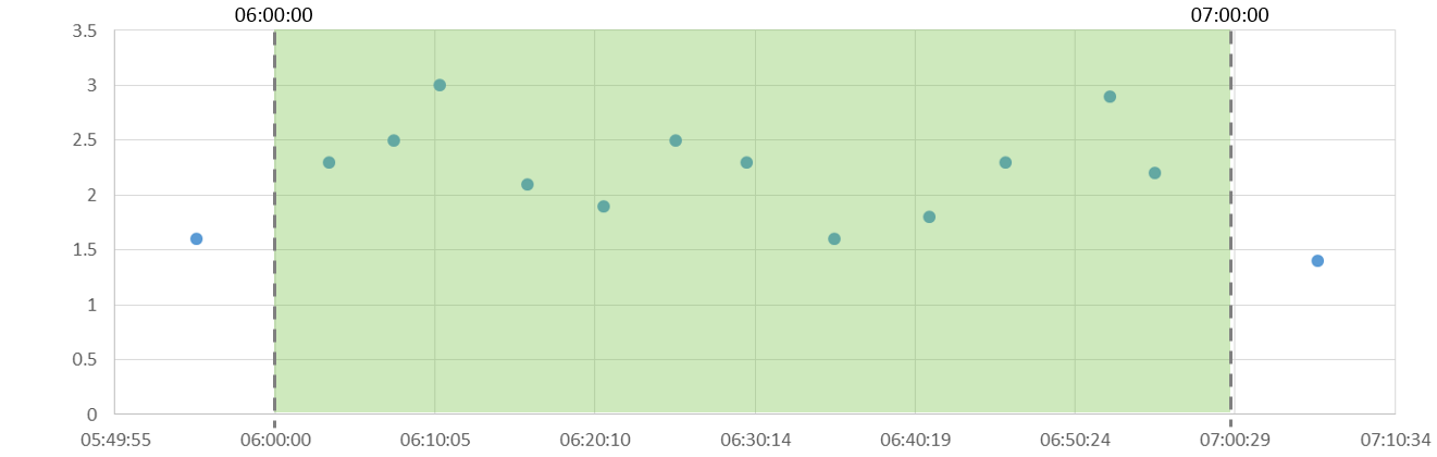
Which, graphically, looks like this if we plot the points. The shaded area is the time period we are interested in for our summary information.
Flow uses a “Stair Step” interpolation between each point, like this:
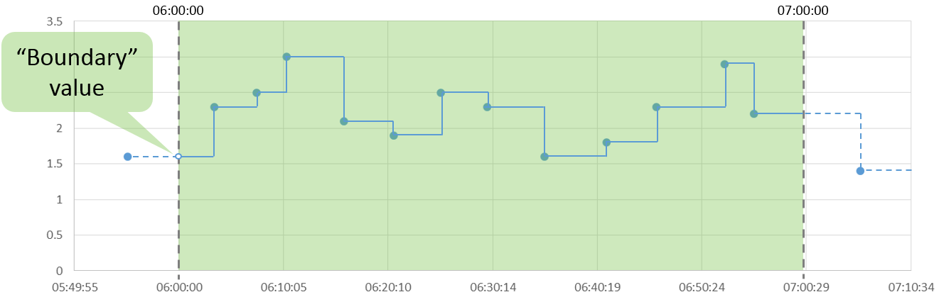
Because the first point in our data set is outside of our summary time period, Flow uses it as a “boundary” value with a timestamp of exactly 06:00:00.
For each time period, you can apply one of the standard aggregation methods on these data points, which will return a single value for that time period. This single value is calculated differently for each of the aggregation methods.